Introduction
cycleTrendR provides a unified framework for analyzing time‑series that contain both trend and cyclic components. It supports:
LOESS, GAM, and GAMM trend estimation
Automatic Fourier harmonic selection (AICc/BIC)
Bootstrap confidence intervals (IID or MBB)
Change‑point detection
Lomb–Scargle periodogram for irregular sampling
Rolling‑origin forecasting
Publication‑quality ggplot2 visualizations
This vignette demonstrates the main workflows using simulated data.
LOESS Trend + Automatic Fourier Selection
res_loess <- adaptive_cycle_trend_analysis(
  signal = signal,
  dates = dates,
  trendmethod = "loess",
  usefourier = TRUE,
  auto_fourier_select = TRUE,
  nboot = 50
)
#> Using original scale.
#> Irregular dates detected: Lomb Scargle + LOESS/GAM(M)
#> Auto seasonality: dominant period approx 20.14 samples -> seasonalfrequency=20
#> loess.as proposed span (criterion=aicc) = 0.944
#> Fourier selection: criterion=AICc -> K=1 (from 0..6)
#> Warning in adaptive_cycle_trend_analysis(signal = signal, dates = dates, :
#> Model-based CI not implemented for this configuration; switching to
#> bootstrapiid.
#> Bootstrap CI (bootstrapiid): 50 resamples
#> Warning in tseries::adf.test(signal, alternative = "stationary"): p-value
#> smaller than printed p-value
#> Warning in tseries::kpss.test(signal, null = "Level"): p-value greater than
#> printed p-value

res_loess$Plot$Trend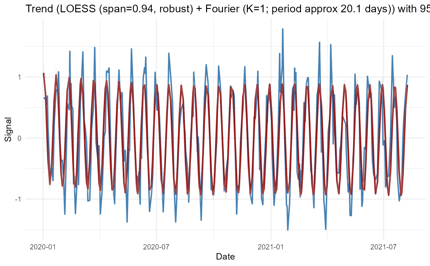
GAM Trend
res_gam <- adaptive_cycle_trend_analysis(
  signal = signal,
  dates = dates,
  trendmethod = "gam",
  usefourier = TRUE,
  nboot = 50
)
#> Using original scale.
#> Irregular dates detected: Lomb Scargle + LOESS/GAM(M)
#> Auto seasonality: dominant period approx 20.14 samples -> seasonalfrequency=20
#> Fourier selection: criterion=AICc -> K=1 (from 0..6)
#> Warning in adaptive_cycle_trend_analysis(signal = signal, dates = dates, :
#> Model-based CI not implemented for this configuration; switching to
#> bootstrapiid.
#> Bootstrap CI (bootstrapiid): 50 resamples
#> Warning in tseries::adf.test(signal, alternative = "stationary"): p-value
#> smaller than printed p-value
#> Warning in tseries::kpss.test(signal, null = "Level"): p-value greater than
#> printed p-value

res_gam$Plot$Trend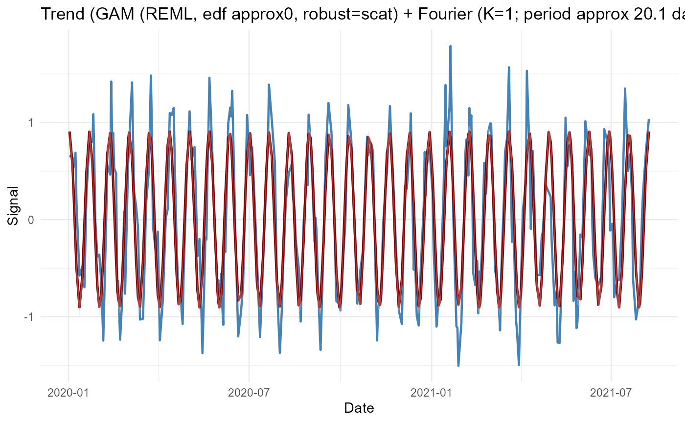
GAMM Trend with Random Effects
group <- rep(letters[1:4], length.out = length(signal))

res_gamm <- adaptive_cycle_trend_analysis(
  signal = signal,
  dates = dates,
  trendmethod = "gam",
  use_gamm = TRUE,
  group_var = "subject",
  group_values = group,
  usefourier = FALSE,
  nboot = 20
)
#> Using original scale.
#> Irregular dates detected: Lomb Scargle + LOESS/GAM(M)
#> Attached grouping column 'subject' from `group_values`.
#> Converted group_var 'subject' to factor (4 levels).
#> Auto seasonality: dominant period approx 20.14 samples -> seasonalfrequency=20
#> Warning in adaptive_cycle_trend_analysis(signal = signal, dates = dates, :
#> Model-based CI not implemented for this configuration; switching to
#> bootstrapiid.
#> Bootstrap CI (bootstrapiid): 20 resamples
#> Warning in tseries::adf.test(signal, alternative = "stationary"): p-value
#> smaller than printed p-value
#> Warning in tseries::kpss.test(signal, null = "Level"): p-value greater than
#> printed p-value

res_gamm$Plot$Trend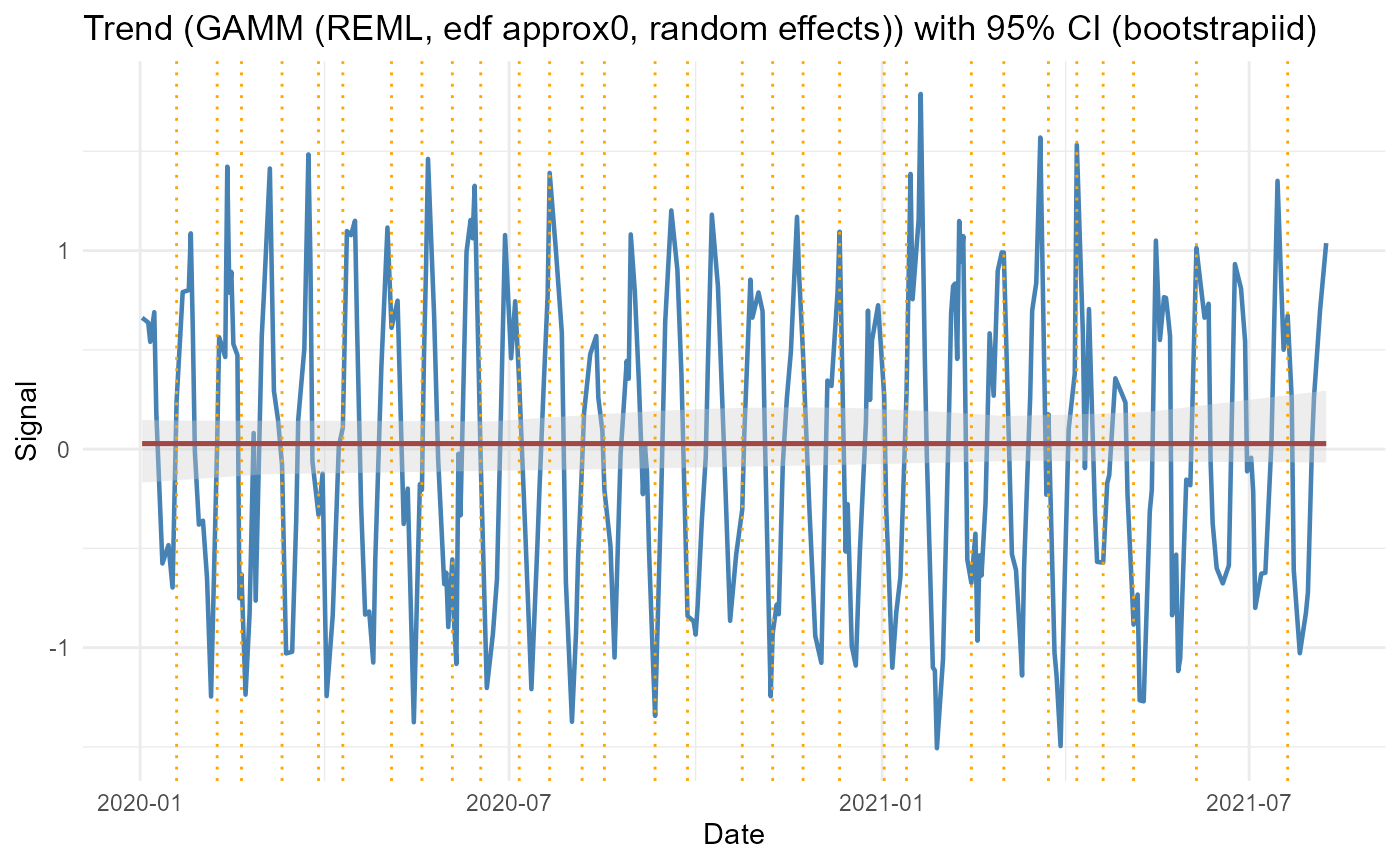
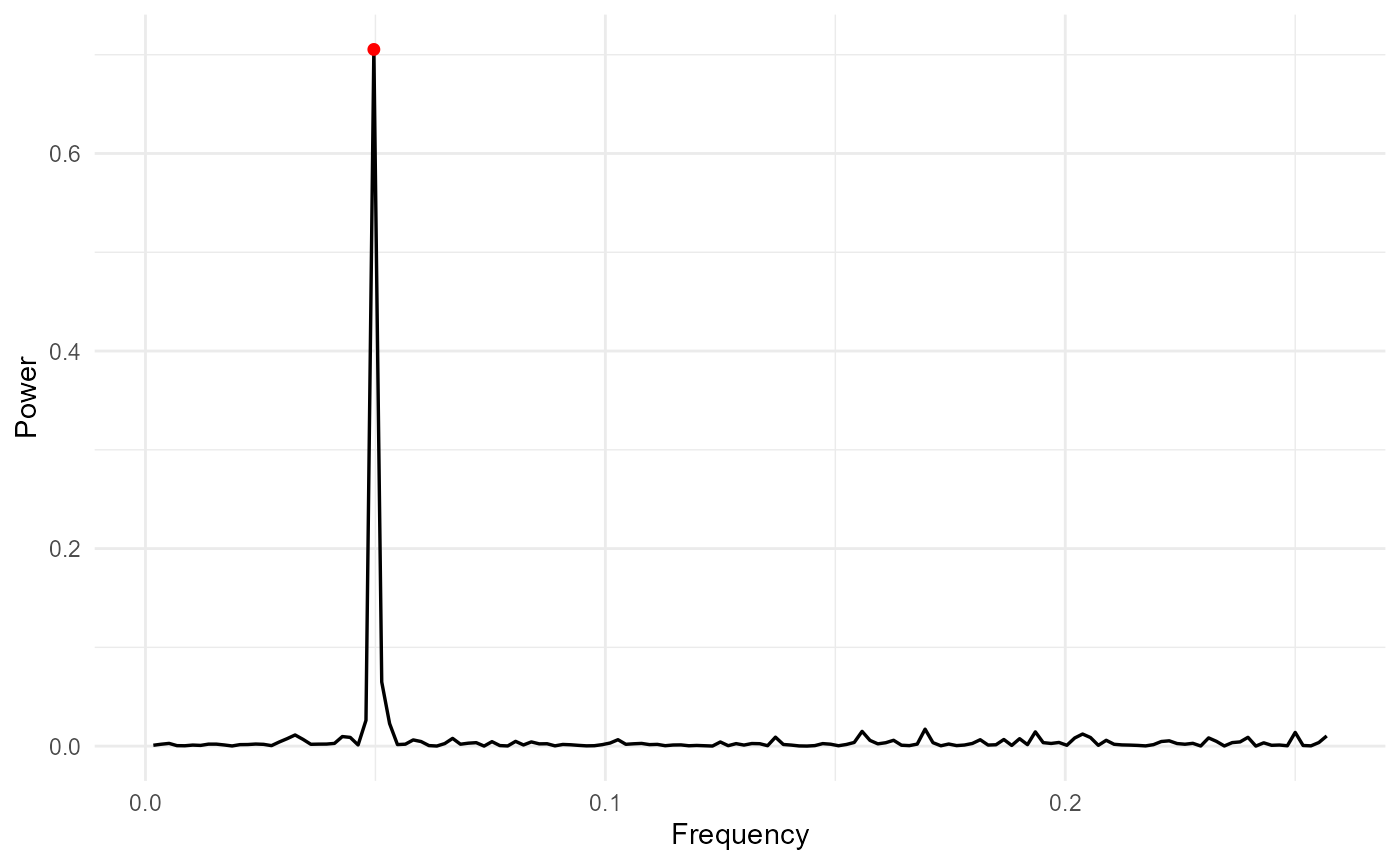
Irregular Sampling + Fourier + Lomb–Scargle
Irregular sampling is detected automatically and the Lomb–Scargle periodogram is used:
  res_irreg <- adaptive_cycle_trend_analysis(
  signal = signal,
  dates = dates,
  trendmethod = "loess",
  usefourier = TRUE,
  auto_fourier_select = TRUE,
  nboot = 50
)
#> Using original scale.
#> Irregular dates detected: Lomb Scargle + LOESS/GAM(M)
#> Auto seasonality: dominant period approx 20.14 samples -> seasonalfrequency=20
#> loess.as proposed span (criterion=aicc) = 0.944
#> Fourier selection: criterion=AICc -> K=1 (from 0..6)
#> Warning in adaptive_cycle_trend_analysis(signal = signal, dates = dates, :
#> Model-based CI not implemented for this configuration; switching to
#> bootstrapiid.
#> Bootstrap CI (bootstrapiid): 50 resamples
#> Warning in tseries::adf.test(signal, alternative = "stationary"): p-value
#> smaller than printed p-value
#> Warning in tseries::kpss.test(signal, null = "Level"): p-value greater than
#> printed p-value

res_irreg$Plot$Spectrum