rareflow: Normalizing Flows for Rare-Event Inference

Introduction

Rare events are outcomes that occur with extremely small probability but often carry significant scientific or practical importance. Examples include:

transitions between metastable states in stochastic differential equations (SDEs),
deviations of empirical distributions from their expected values,
failure events in complex systems,
tail events in biological, physical, or financial models.

Estimating rare-event probabilities is challenging because:

naïve Monte Carlo requires an enormous number of samples,
the relevant trajectories are atypical,
the underlying dynamics may be high-dimensional or nonlinear.

rareflow provides a unified framework that combines:

Sanov theory for empirical distributions,

Girsanov change of measure for SDEs,

Freidlin–Wentzell large deviations for small-noise diffusions,

with normalizing flows for flexible variational inference.

The package offers modular flow models, variational optimization, and specialized wrappers for rare-event tilting.

1.A first example: variational inference for a discrete rare event

We consider an observed empirical distribution:

Qobs <- c(0.05, 0.90, 0.05)
px <- function(z) c(0.3, 0.4, 0.3)

We construct a planar flow and fit a variational posterior:

flow <- makeflow("planar", list(u = 0.1, w = 0.2, b = 0))
fit <- fitflowvariational(Qobs, pxgivenz = px, nmc = 500)
fit$elbo
#> [1] -0.9438972

This computes the Evidence Lower Bound (ELBO):

2. Girsanov tilting for SDEs

Consider the SDE:

We simulate Brownian increments:

b <- function(x) -x
dt <- 0.01
T <- 1000
set.seed(1)
Winc <- rnorm(T, sd = sqrt(dt))

Define a drift tilt:

theta <- rep(0.5, T)
girsanov_logratio(theta, Winc, dt)
#> [1] -1.832407

We can fit a tilted variational model using the wrapper:

set.seed(123)
dt  <- 0.01
T   <- 1000
Winc <- rnorm(T, sd = sqrt(dt))
theta_path <- rep(0, length(Winc))
fit_gir <- fitflow_girsanov(
  observed      = Qobs,
  base_pxgivenz = px,
  theta_path    = theta_path,
  Winc          = Winc,
  dt            = dt
)

3. Freidlin–Wentzell quasi-potential

For small-noise diffusions of the form:

$dX_t = b(X_t)\, dt + \sqrt{\varepsilon}\, dW_t,$

rare transitions are governed by the Freidlin–Wentzell action:

$S[x] = \frac{1}{2} \int_0^T \| x'(t) - b(x(t)) \|^2 \, dt.$

Double-well potential

The classical double-well potential is

$V(x) = \frac{x^4}{4} - \frac{x^2}{2},$

with drift

$b(x) = -V'(x) = x - x^3.$

We visualize the potential landscape:

V <- function(x) x^4/4 - x^2/2
xs <- seq(-2, 2, length.out = 400)

plot(xs, V(xs), type = "l", lwd = 2,
     main = "Double-Well Potential",
     ylab = "V(x)", xlab = "x")
abline(v = c(-1, 1), lty = 3, col = "gray")

The quasi-potential between two points $a$ and $b$ is defined as the minimum action over all admissible paths connecting them:

$V(a, b) = \inf_{x(0)=a,\, x(T)=b} S[x].$

We compute the quasi-potential between two points:

b<- function(x) {
  v<- as.numeric(x)
  return(c(v - v^3)) #double-well drift
}
qp<- FW_quasipotential(-1, 1, drift = b, T = 200, dt = 0.01)
qp$action
#> [1] 132900.4

Plot the minimum-action path:

plot(qp$path, type = "l", main = "Minimum-Action Path (Freidlin–Wentzell)")

3.1 Two-dimensional example: radial double-well

We consider the 2D potential

$V(x,y) = \frac{1}{4}(x^2 + y^2 - 1)^2,$

whose minima form a ring of radius 1.
The drift is

$b(x,y) = -(x^2 + y^2 - 1)(x, y).$

We visualize the potential landscape:

V2 <- function(x, y) 0.25 * (x^2 + y^2 - 1)^2

xs <- seq(-2, 2, length.out = 200)
ys <- seq(-2, 2, length.out = 200)
grid <- expand.grid(x = xs, y = ys)
Z <- matrix(V2(grid$x, grid$y), nrow = length(xs))

contour(xs, ys, Z,
        nlevels = 20,
        main = "2D Radial Double-Well Potential",
        xlab = "x", ylab = "y")

We simulate a 2D diffusion:

$dX_t = b(X_t)\, dt + \sqrt{\varepsilon}\, dW_t.$

dt <- 0.01
T <- 5000
x <- matrix(0, nrow = T, ncol = 2)

b2 <- function(v) {
  r2 <- sum(v^2)
  -(r2 - 1) * v
}

for (t in 1:(T-1)) {
  drift <- b2(x[t, ])
  noise <- sqrt(dt) * rnorm(2)
  x[t+1, ] <- x[t, ] + drift * dt + noise
}

plot(x[,1], x[,2], type = "l",
     main = "2D Diffusion in a Radial Double-Well",
     xlab = "x", ylab = "y")

3.2 Minimum Action Path in 2D (String Method)

We compute a 2D Freidlin–Wentzell minimum-action path using a simple string-method iteration.

We consider the radial double-well potential:

$V(x,y) = \frac{1}{4}(x^2 + y^2 - 1)^2, \qquad b(x,y) = -\nabla V(x,y) = -(x^2 + y^2 - 1)(x, y).$

We compute a MAP between the points $(-1,0)$ and $(1,0)$ .

# Potential and drift
V2 <- function(x, y) 0.25 * (x^2 + y^2 - 1)^2
b2 <- function(v) {
  r2 <- sum(v^2)
  -(r2 - 1) * v
}

# String method parameters
N <- 80          # number of points in the string
steps <- 200     # number of iterations
dt_sm <- 0.01    # step size

# Initial straight-line path
path <- cbind(seq(-1, 1, length.out = N), rep(0, N))

# String method iterations
for (k in 1:steps) {
  # Update each interior point
  for (i in 2:(N-1)) {
    drift <- b2(path[i, ])
    path[i, ] <- path[i, ] + dt_sm * drift
  }
  
  # Reparametrize to keep points evenly spaced
  d <- sqrt(rowSums(diff(path)^2))
  s <- c(0, cumsum(d))
  s <- s / max(s)
  path <- cbind(
    approx(s, path[,1], xout = seq(0,1,length.out=N))$y,
    approx(s, path[,2], xout = seq(0,1,length.out=N))$y
  )
}

plot(path[,1], path[,2], type="l", lwd=2,
     main="2D Minimum Action Path (String Method)",
     xlab="x", ylab="y")
points(c(-1,1), c(0,0), pch=19, col="red")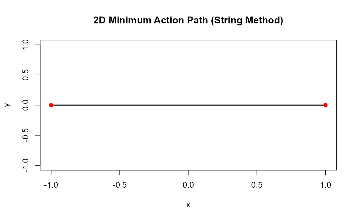

library(ggplot2)
library(gganimate)
#> No renderer backend detected. gganimate will default to writing frames to separate files
#> Consider installing:
#> - the `gifski` package for gif output
#> - the `av` package for video output
#> and restarting the R session

3.3 Animation of a 2D diffusion trajectory

We animate the 2D trajectory simulated in the radial double-well potential.

# Simulate a 2D trajectory
dt <- 0.01
T <- 2000
x <- matrix(0, nrow = T, ncol = 2)

for (t in 1:(T-1)) {
  drift <- b2(x[t, ])
  noise <- sqrt(dt) * rnorm(2)
  x[t+1, ] <- x[t, ] + drift * dt + noise
}

df <- data.frame(
  t = 1:T,
  x = x[,1],
  y = x[,2]
)

p <- ggplot(df, aes(x, y)) +
  geom_path(alpha = 0.4) +
  geom_point(aes(frame = t), color = "red", size = 2) +
  coord_equal() +
  labs(title = "2D Diffusion Trajectory", x = "x", y = "y")

animate(p, nframes = 200, fps = 20)

4. Full workflow: bistable diffusion and rare-event estimation

We simulate a bistable diffusion:

b <- function(x) x - x^3
dt <- 0.01
T <- 2000
x <- numeric(T)
for (t in 1:(T-1)) {
  x[t+1] <- x[t] + b(x[t])*dt + sqrt(dt)*rnorm(1)
}

Define a rare event: reaching the right well.

rare_event <- mean(x > 1.5)
rare_event
#> [1] 0.0505

Construct an empirical distribution:

Qobs <- c(mean(x < -0.5), mean(abs(x) <= 0.5), mean(x > 0.5))
px <- function(z) c(0.3, 0.4, 0.3)

Fit a variational flow:

fit <- fitflowvariational(Qobs, pxgivenz = px)
fit$elbo
#> [1] -1.127451

Conclusions

rareflow provides:

a unified interface for rare-event modeling,
modular normalizing flows,
variational inference tools,
Girsanov and Freidlin–Wentzell utilities.

Future extensions may include:

minimum action method (MAM),
string method,
multidimensional examples,
built-in datasets.

References

Dembo, A., & Zeitouni, O. (1998). Large Deviations Techniques and Applications. Springer.
Oksendal, B. (2003). Stochastic Differential Equations: An Introduction with Applications. Springer.
Freidlin, M. I., & Wentzell, A. D. (2012). Random Perturbations of Dynamical Systems. Springer.

Pietro